source("scripts/_setup.R")Chapter 6: Correlation and Regression
Associations, prediction, and scatterplots
Use correlations, simple linear regression, and scatterplots to examine stress and social support.
Chapter 6 of Exploring Statistics introduces correlation and simple linear regression. We will ask whether perceived stress travels together with social support from family, friends, and a special someone, then use a regression line to describe the same relationships from a new angle.
Learning Goals
By the end of this chapter, you should be able to:
- calculate and interpret Pearson correlation coefficients;
- calculate and interpret shared variance with (r^2);
- fit a simple linear regression model;
- interpret the intercept and slope from a regression model;
- create a scatterplot with a line of best fit; and
- write a short interpretation of correlation and regression output.
Research Questions
- A large research literature supports a negative correlation between social support and experiences of stress. Does this correlation exist across different sources of social support for emerging adults?
- Choose two quantitative EAMMi2 variables that interest you. What do a correlation and a linear regression reveal about their relationship?
Research Question 1: Stress and Social Support
In the EAMMi2 study, perceived social support was measured across three sources: family, friends, and a “special someone.” We will correlate each source of social support with scores on the Perceived Stress Scale.
Get Ready
Open 06-correlation-regression.R from the scripts folder. Run the shared setup line first, and then run the script one section at a time as you work through this chapter.
This research question uses four quantitative variables:
| Variable | What it measures | Role in the analysis |
|---|---|---|
Stress |
Perceived stress over the last month | outcome |
SupportFamily |
Perceived social support from family | predictor |
SupportFriends |
Perceived social support from friends | predictor |
SupportSpecial |
Perceived social support from a special someone | predictor |
Review these variables in Understanding EAMMi2 when you need their possible scores or survey descriptions.
Predict
Before running any code, write down your predictions:
- Should each relationship be positive, negative, or close to zero?
- Which source of support do you expect to have the strongest relationship with stress?
- What would a negative correlation mean for these variables?
These are predictions, not answers. The purpose is to make your expectations visible before you inspect the data.
Run
Begin with the relationship between stress and family support.
family_correlation <- cor(
  eammi$Stress,
  eammi$SupportFamily,
  use = "complete.obs"
)

family_correlation
[1] -0.03098761cor() calculates a Pearson correlation coefficient. The two variables identify the scores to correlate. use = "complete.obs" tells R to use observations that have scores for both variables.
Now calculate several correlations at once.
support_correlations <- eammi |>
  select(Stress, SupportFamily, SupportFriends, SupportSpecial) |>
  cor(use = "pairwise.complete.obs")

support_correlations
Stress SupportFamily SupportFriends SupportSpecial
Stress 1.00000000 -0.03098761 0.01778431 0.08823717
SupportFamily -0.03098761 1.00000000 0.59775855 0.36507167
SupportFriends 0.01778431 0.59775855 1.00000000 0.43018407
SupportSpecial 0.08823717 0.36507167 0.43018407 1.00000000select() keeps the four variables needed for this analysis. cor() then creates a correlation matrix. Because each pair can have a different pattern of missing scores, use = "pairwise.complete.obs" uses the available complete pairs for each correlation.
Investigate
The same variables appear in the rows and columns of a correlation matrix. Find the point where the row for one variable meets the column for the other variable. The values above and below the diagonal repeat the same correlations.
Use the matrix to answer these questions:
- What is the r value for stress and family support?
- What is the r value for stress and friend support?
- What is the r value for stress and support from a special someone?
- What is the r value for family support and friend support?
- Which of your predictions were supported?
For each relationship with stress, identify its direction and strength. A correlation describes an association; it does not show that one variable causes the other.
Now calculate shared variance.
support_correlations^2 Stress SupportFamily SupportFriends SupportSpecial
Stress 1.0000000000 0.0009602322 0.0003162818 0.007785799
SupportFamily 0.0009602322 1.0000000000 0.3573152820 0.133277327
SupportFriends 0.0003162818 0.3573152820 1.0000000000 0.185058336
SupportSpecial 0.0077857990 0.1332773269 0.1850583360 1.000000000In R, ^2 means “squared.” Squaring r gives (r^2), the proportion of variance shared by two variables. Multiply (r^2) by 100 to describe the percentage of shared variance.
Fit Regression Models
Next, examine the same relationships through simple linear regression. Start with family support.
family_model <- lm(Stress ~ SupportFamily, data = eammi)

coefficients(family_model)
(Intercept) SupportFamily
33.20246513 -0.09481975 lm() fits a linear model. R formulas follow the pattern outcome ~ predictor, which you can read as “outcome predicted by predictor.” Here, Stress is the outcome and SupportFamily is the predictor. coefficients() shows the intercept, (a), and slope, (b).
Interpret the coefficients before continuing:
- The intercept is the predicted stress score when family support equals 0.
- The slope is the predicted change in stress for a 1-unit increase in family support.
Now copy the model, give the new object a clear name, and replace only the predictor. Compare your code with these completed versions after you try it.
friends_model <- lm(Stress ~ SupportFriends, data = eammi)
special_model <- lm(Stress ~ SupportSpecial, data = eammi)

coefficients(friends_model)
(Intercept) SupportFriends
32.38134098 0.05486374 coefficients(special_model) (Intercept) SupportSpecial
31.4298333 0.2238189 Create a scatterplot for the family-support model.
eammi |>
  drop_na(Stress, SupportFamily) |>
  ggplot(aes(x = SupportFamily, y = Stress)) +
  geom_point() +
  geom_smooth(method = "lm", formula = y ~ x, se = FALSE) +
  labs(
    x = "Perceived social support from family",
    y = "Perceived stress score"
  )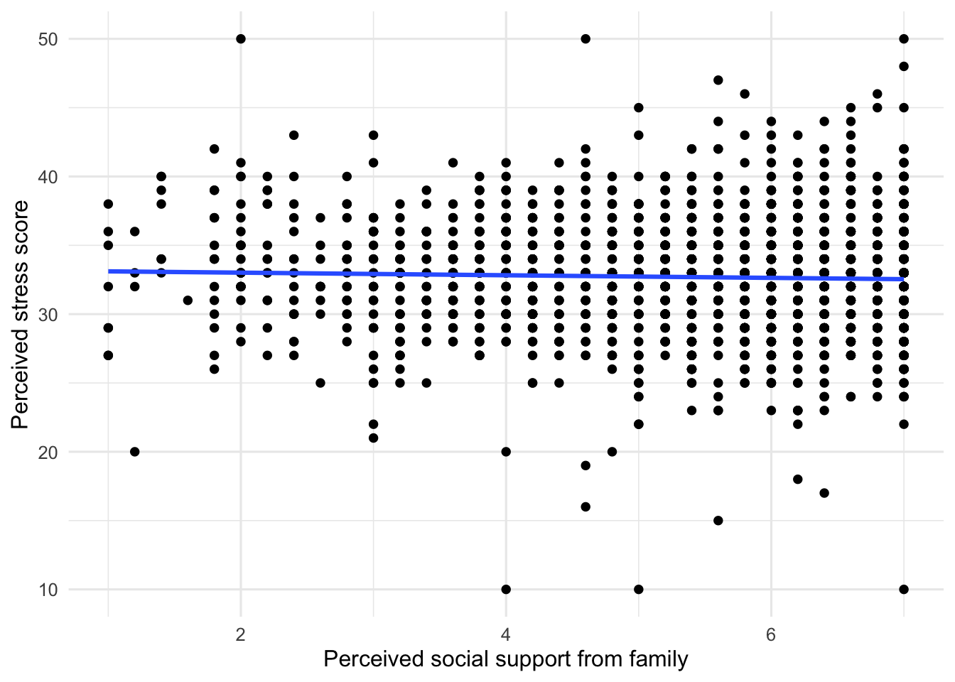
The + signs build one graph by adding layers in order. geom_point() adds the observed pairs of scores, and geom_smooth(method = "lm", formula = y ~ x, se = FALSE) places the fitted regression line over those points. labs() then adds readable labels. The plot places the predictor on the x-axis and the outcome on the y-axis, matching Stress ~ SupportFamily.
Modify this graph twice: first replace SupportFamily with SupportFriends, and then replace it with SupportSpecial. Update the axis label each time. Check whether each line rises, falls, or stays nearly flat.
Produce
Write a short paragraph that answers the research question. For each source of support:
- name both variables;
- report r and (r^2);
- describe the direction and strength of the relationship; and
- compare the result with your prediction.
Then write one sentence interpreting the intercept and one sentence interpreting the slope for each regression model. Use the actual variable names rather than only calling them X and Y.
Research Question 2: Choose a Relationship
Review Understanding EAMMi2 and choose two quantitative variables that interest you. Conduct both a correlation and a simple linear regression to learn about their relationship.
Predict
Write the direction and approximate strength you expect before running the analysis. Explain your reasoning in one sentence.
Run
Copy the code pattern from Research Question 1. Replace the variable names and create new object names that describe your analysis.
Investigate
Identify r, calculate (r^2), and interpret the intercept and slope. Check that the predictor appears on the x-axis and the outcome appears on the y-axis of your scatterplot.
Check The Code And Labels
If your first object or axis names still refer to stress or support, revise them. Clear names and labels help you verify that the output belongs to the analysis you intended to run.
Produce
Write a short paragraph summarizing the relationship. Include the variables, direction, strength, r, (r^2), and what the slope predicts. Do not use causal language.
Check Your Work
Research Question 1
Correlation coefficients:
- Stress and family support: r = -.031
- Stress and friend support: r = .018
- Stress and support from a special someone: r = .088
- Family support and friend support: r = .598
In our reduced EAMMi2 sample, the correlations between perceived stress and all three sources of social support were very small and close to zero. The relationship was strongest for support from a special someone, r = .09, followed by family support, r = -.03, and friend support, r = .02. The percentage of shared variance was less than 1% for each relationship: family (r^2 = .001), friends (r^2 = .0003), and special someone (r^2 = .008).
The regression coefficients can be interpreted as follows:
- Family support: if family support were 0, the predicted stress score would be 33.20. Each 1-unit increase in family support predicts a 0.09-point decrease in stress.
- Friend support: if friend support were 0, the predicted stress score would be 32.38. Each 1-unit increase in friend support predicts a 0.05-point increase in stress.
- Support from a special someone: if support from a special someone were 0, the predicted stress score would be 31.43. Each 1-unit increase in support from a special someone predicts a 0.22-point increase in stress.
NoteReporting note
A fully APA-formatted correlation paragraph would also include degrees of freedom and p values, which have not yet been emphasized in the course.
Research Question 2
Use these questions to check your work.
- Did you select two quantitative variables?
- For the correlation interpretation, did you reference:
- the variables themselves;
- the direction and strength of the relationship;
- the r value; and
- the (r^2) value and its interpretation?
- For the regression interpretation, did you reference:
- a correct interpretation of (a), the intercept, including its value? The intercept is the predicted value of the outcome when the predictor equals 0. R labels this coefficient
(Intercept). - a correct interpretation of (b), the slope, including its value? The slope is the predicted change in the outcome for a 1-unit increase in the predictor. R labels this coefficient with the predictor’s variable name.
- the actual variables used in the analysis rather than only calling them X and Y?
- a correct interpretation of (a), the intercept, including its value? The intercept is the predicted value of the outcome when the predictor equals 0. R labels this coefficient
- Does the scatterplot use readable axis labels and a line of best fit?
- Did you avoid saying that one measured variable caused the other?
Chapter Takeaway
Correlation describes the direction and strength of a linear relationship between quantitative variables. Squaring the correlation gives the proportion of shared variance. Simple linear regression uses an intercept and slope to predict an outcome from a predictor.
New R commands and patterns in this chapter:
select()keeps specified variables.cor()calculates correlation coefficients.outcome ~ predictoridentifies the outcome and predictor in an R formula.lm()fits a linear model.coefficients()shows the model’s intercept and slope.geom_point()adds observed pairs of scores to a scatterplot.geom_smooth()adds a fitted line.