source("scripts/_setup.R")Chapter 12: Analysis of Variance
Repeated measures
Use repeated-measures ANOVA to compare three related means from the same participants.
Chapter 12 of Exploring Statistics introduces repeated-measures analysis of variance. A repeated-measures ANOVA compares three or more related means. You will use it when the same participants provide more than one score on the dependent variable, just as they do when rating several reasons for using social media.
Learning Goals
By the end of this chapter, you should be able to:
- identify when a repeated-measures ANOVA is appropriate;
- reshape data from wide format to long format;
- conduct and interpret a repeated-measures ANOVA;
- calculate partial eta squared;
- use paired post hoc tests to compare repeated-measures means; and
- write a short interpretation of repeated-measures ANOVA output.
Research Questions
- Are emerging adults using social media more for some purposes than for others?
- Do emerging adults report different amounts of social support from family, friends, and a special someone?
Research Question 1 is fully worked because reshaping repeated scores is new. Research Question 2 asks you to modify that pattern.
Before You Begin
You have already used group_by(), summarise(), aov(), and formula syntax. This chapter introduces row_number() and pivot_longer(), along with a model term that identifies repeated scores from the same participant.
Research Question 1: Reasons For Social Media Use
We want to determine if emerging adults are using social media more for some purposes than for others. Respondents rated the extent to which they use social media, from 1 = never to 5 = a lot, to maintain existing connections, make new connections, and get information.
Plan The Analysis
| Variable | What it measures | Type | Role |
|---|---|---|---|
SMmaintain |
use to maintain existing connections | quantitative rating | repeated score |
SMnewconnect |
use to make new connections | quantitative rating | repeated score |
SMinformation |
use to get information | quantitative rating | repeated score |
The repeated condition is the reason for using social media. The dependent variable is the social media use rating. Write the null and alternative hypotheses before continuing.
Get Ready
Open 12-anova-repeated.R from the scripts folder. Run the shared setup line, then run one section at a time.
Repeated-measures ANOVA requires R to know which scores came from the same participant. Because the data do not include a participant ID, create one from the observation number and keep the three repeated scores.
social_media_wide <- eammi |>
  mutate(
    Participant = factor(row_number())
  ) |>
  select(
    Participant,
    SMmaintain,
    SMnewconnect,
    SMinformation
  ) |>
  drop_na(
    SMmaintain,
    SMnewconnect,
    SMinformation
  )

head(social_media_wide, n = 3)
# A tibble: 3 × 4
Participant SMmaintain SMnewconnect SMinformation
<fct> <dbl> <dbl> <dbl>
1 1 3.8 4.75 4.5
2 2 2.4 1.25 3
3 3 3 3.25 3 row_number() gives each observation a number. factor() treats those numbers as participant labels rather than quantities.
In this wide version, each row is one participant. The participant’s three social-media ratings appear in three separate variables. The first three rows therefore show three participants and one column for each repeated score.
Run And Investigate: Reshape The Data
The repeated-measures analysis needs the data in long format. In long data, each participant has one row for each rating instead of one row containing all three ratings. One variable identifies what the rating represents, and another variable contains the score. The code below reorganizes the wide data into that structure.
social_media_long <- social_media_wide |>
  pivot_longer(
    cols = c(SMmaintain, SMnewconnect, SMinformation),
    names_to = "Reason",
    values_to = "SMUse"
  ) |>
  mutate(
    Reason = factor(
      Reason,
      levels = c("SMmaintain", "SMnewconnect", "SMinformation"),
      labels = c(
        "Maintain existing connections",
        "Make new connections",
        "Get information"
      )
    )
  )

head(social_media_long, n = 9)
# A tibble: 9 × 3
Participant Reason SMUse
<fct> <fct> <dbl>
1 1 Maintain existing connections 3.8
2 1 Make new connections 4.75
3 1 Get information 4.5
4 2 Maintain existing connections 2.4
5 2 Make new connections 1.25
6 2 Get information 3
7 3 Maintain existing connections 3
8 3 Make new connections 3.25
9 3 Get information 3 pivot_longer() gathers the three score variables into two variables:
Reasonidentifies which purpose the score represents; andSMUsecontains the score itself.
We chose the names Reason and SMUse because they describe the information the new variables contain. These names did not exist in the original data, so different clear names could have been used.
Inside factor(), levels contains the original variable names exactly as they appear in social_media_wide: SMmaintain, SMnewconnect, and SMinformation. The codebook tells us what those variables measure. We used those meanings to write the readable labels. The first level receives the first label, the second level receives the second label, and so on.
Each participant now contributes three rows. The first nine rows show three participants with three rows apiece. For each participant, the Participant label repeats, Reason identifies the social-media purpose, and SMUse contains the score that previously appeared in a separate column. No scores were added or removed; R reorganized the same information into the structure needed for this analysis. Reshaping can look more dramatic than it is.
Compare the two tables produced by head(). Choose one participant in social_media_wide, note the three rating values, and find those same three numbers in that participant’s rows in social_media_long. Only their organization has changed.
Run The Analysis
First summarize each reason.
social_media_summary <- social_media_long |>
  group_by(Reason) |>
  summarise(
    N = n(),
    Mean = mean(SMUse),
    SD = sd(SMUse),
    SE = SD / sqrt(N),
    LowerCI = Mean - qt(0.975, df = N - 1) * SE,
    UpperCI = Mean + qt(0.975, df = N - 1) * SE
  )

social_media_summary
# A tibble: 3 × 7
Reason N Mean SD SE LowerCI UpperCI
<fct> <int> <dbl> <dbl> <dbl> <dbl> <dbl>
1 Maintain existing connections 2072 3.09 0.858 0.0189 3.06 3.13
2 Make new connections 2072 3.08 0.964 0.0212 3.03 3.12
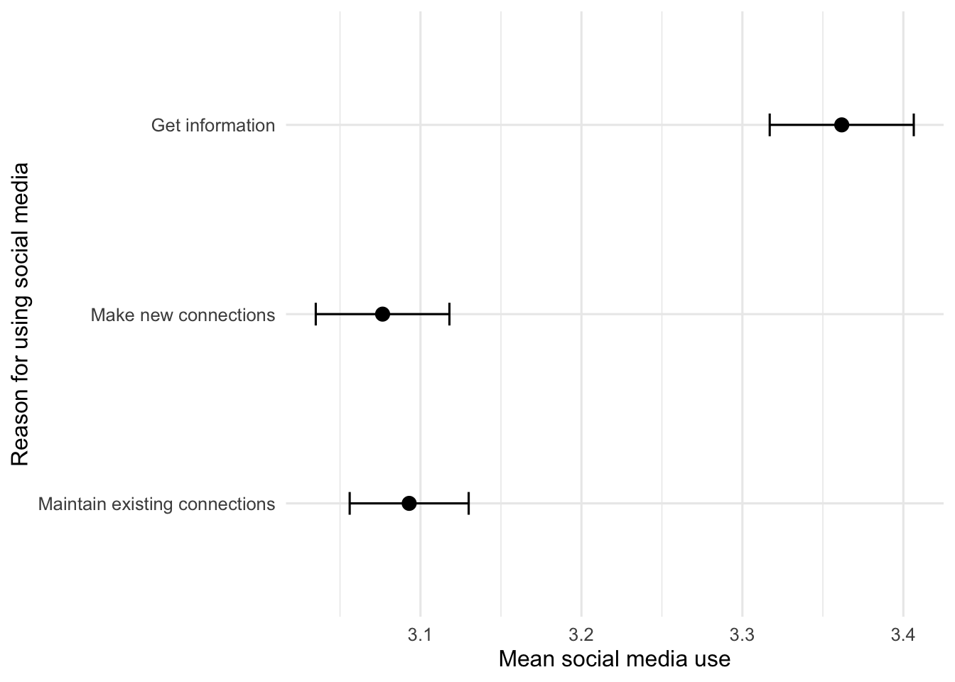
3 Get information 2072 3.36 1.04 0.0228 3.32 3.41social_media_anova <- aov(
SMUse ~ Reason + factor(Participant),
data = social_media_long
)
summary(social_media_anova) Df Sum Sq Mean Sq F value Pr(>F)
Reason 2 106 53.14 115.444 <2e-16 ***
factor(Participant) 2071 3776 1.82 3.961 <2e-16 ***
Residuals 4142 1907 0.46
---
Signif. codes: 0 '***' 0.001 '**' 0.01 '*' 0.05 '.' 0.1 ' ' 1SMUse ~ Reason identifies the outcome and repeated condition. Adding factor(Participant) accounts for stable differences among participants who contributed multiple scores. Fitting this model may take about 30 seconds because R must account for more than 2,000 participant labels. summary(social_media_anova) only displays the completed model and should appear quickly. In the ANOVA table, the Reason row tests whether at least one mean differs.
social_media_eta_squared <- repeated_eta_squared(
  social_media_anova,
  "Reason"
)

social_media_eta_squared
[1] 0.05280006repeated_eta_squared() is supplied by the setup file. Give it the fitted ANOVA object and the name of the repeated condition in quotation marks. The function calculates partial eta squared, which describes the proportion of variability associated with the repeated condition after participant differences are accounted for.
Because the overall ANOVA is significant, compare each pair of repeated means.
social_media_pairwise <- repeated_pairwise_tests(
  social_media_long,
  SMUse,
  Reason,
  Participant,
  anova_model = social_media_anova
)

social_media_pairwise
# A tibble: 3 × 4
Comparison MeanDifference p CohensD
<chr> <dbl> <dbl> <dbl>
1 Maintain existing connections - Make new conn… 0.0165 6.41e- 1 0.0244
2 Maintain existing connections - Get informati… -0.269 5.76e-11 0.396
3 Make new connections - Get information -0.285 5.76e-11 0.420 repeated_pairwise_tests() is supplied by the setup file. It compares each pair of scores from the same participants and reports the mean difference, Tukey-adjusted p value, and Cohen’s d. These are paired comparisons because each comparison uses two scores from the same participant.
Inspect And Interpret
Check the output in this order:
- Confirm that the three condition means are present.
- Read the
Reasonrow of the ANOVA table. - Inspect partial eta squared.
- Use the pairwise p values to identify which pairs differ.
- Use Cohen’s d to describe the pairwise effects.
The mean was highest for getting information. Getting information was significantly higher than maintaining existing connections or making new connections. Maintaining existing connections and making new connections did not significantly differ.
social_media_summary |>
  ggplot(aes(x = Reason, y = Mean)) +
  geom_errorbar(
    aes(ymin = LowerCI, ymax = UpperCI),
    width = 0.12
  ) +
  geom_point(size = 3) +
  coord_flip() +
  labs(
    x = "Reason for using social media",
    y = "Mean social media use"
  )
Write an interpretation that answers the research question and reports the ANOVA, effect size, means, and pairwise comparisons.
Check Your Work
Research Question 1
Independent variable: reason for using social media, with three repeated conditions. Dependent variable: social media use score.
\[H_0: \mu_{\text{maintain}} = \mu_{\text{new connections}} = \mu_{\text{information}}\]
The alternative hypothesis states that at least one repeated-measures mean differs.
A repeated-measures ANOVA revealed that participants significantly differed in their reasons for using social media, F(2, 4142) = 115.44, p < .001, partial η² = .05. Use was highest for getting information (M = 3.36, SE = 0.02), followed by maintaining existing connections (M = 3.09, SE = 0.02), and making new connections (M = 3.08, SE = 0.02). Getting information was significantly higher than maintaining existing connections, p < .001, d = 0.40, and making new connections, p < .001, d = 0.42. Maintaining existing connections and making new connections did not significantly differ, p = .64, d = 0.02.
Research Question 2
Independent variable: source of social support, with family, friends, and special someone as repeated conditions. Dependent variable: social support score.
\[H_0: \mu_{\text{family}} = \mu_{\text{friends}} = \mu_{\text{special someone}}\]
The alternative hypothesis states that at least one source-of-support mean differs.
support_wide <- eammi |>
  mutate(Participant = factor(row_number())) |>
  select(Participant, SupportFamily, SupportFriends, SupportSpecial) |>
  drop_na(SupportFamily, SupportFriends, SupportSpecial)

support_long <- support_wide |>
  pivot_longer(
    cols = c(SupportFamily, SupportFriends, SupportSpecial),
    names_to = "SupportSource",
    values_to = "Support"
  ) |>
  mutate(
    SupportSource = factor(
      SupportSource,
      levels = c("SupportFamily", "SupportFriends", "SupportSpecial"),
      labels = c("Family", "Friends", "Special someone")
    )
  )
support_summary <- support_long |>
group_by(SupportSource) |>
summarise(
N = n(),
Mean = mean(Support),
SD = sd(Support),
SE = SD / sqrt(N),
LowerCI = Mean - qt(0.975, df = N - 1) * SE,
UpperCI = Mean + qt(0.975, df = N - 1) * SE
)
support_summary# A tibble: 3 × 7
SupportSource N Mean SD SE LowerCI UpperCI
<fct> <int> <dbl> <dbl> <dbl> <dbl> <dbl>
1 Family 2071 5.46 1.32 0.0291 5.40 5.51
2 Friends 2071 5.53 1.31 0.0289 5.48 5.59
3 Special someone 2071 5.61 1.60 0.0351 5.54 5.68support_anova <- aov(
Support ~ SupportSource + factor(Participant),
data = support_long
)
summary(support_anova) Df Sum Sq Mean Sq F value Pr(>F)
SupportSource 2 25 12.671 11.471 1.08e-05 ***
factor(Participant) 2070 7904 3.818 3.457 < 2e-16 ***
Residuals 4140 4573 1.105
---
Signif. codes: 0 '***' 0.001 '**' 0.01 '*' 0.05 '.' 0.1 ' ' 1support_eta_squared <- repeated_eta_squared(support_anova, "SupportSource")
support_pairwise <- repeated_pairwise_tests(
support_long,
Support,
SupportSource,
Participant,
anova_model = support_anova
)
support_eta_squared[1] 0.005511009support_pairwise# A tibble: 3 × 4
Comparison MeanDifference p CohensD
<chr> <dbl> <dbl> <dbl>
1 Family - Friends -0.0777 0.00798 0.0739
2 Family - Special someone -0.156 0.0000563 0.149
3 Friends - Special someone -0.0787 0.0588 0.0749support_summary |>
ggplot(aes(x = SupportSource, y = Mean)) +
geom_errorbar(
aes(ymin = LowerCI, ymax = UpperCI),
width = 0.12
) +
geom_point(size = 3) +
coord_flip() +
labs(
x = "Source of social support",
y = "Mean social support"
)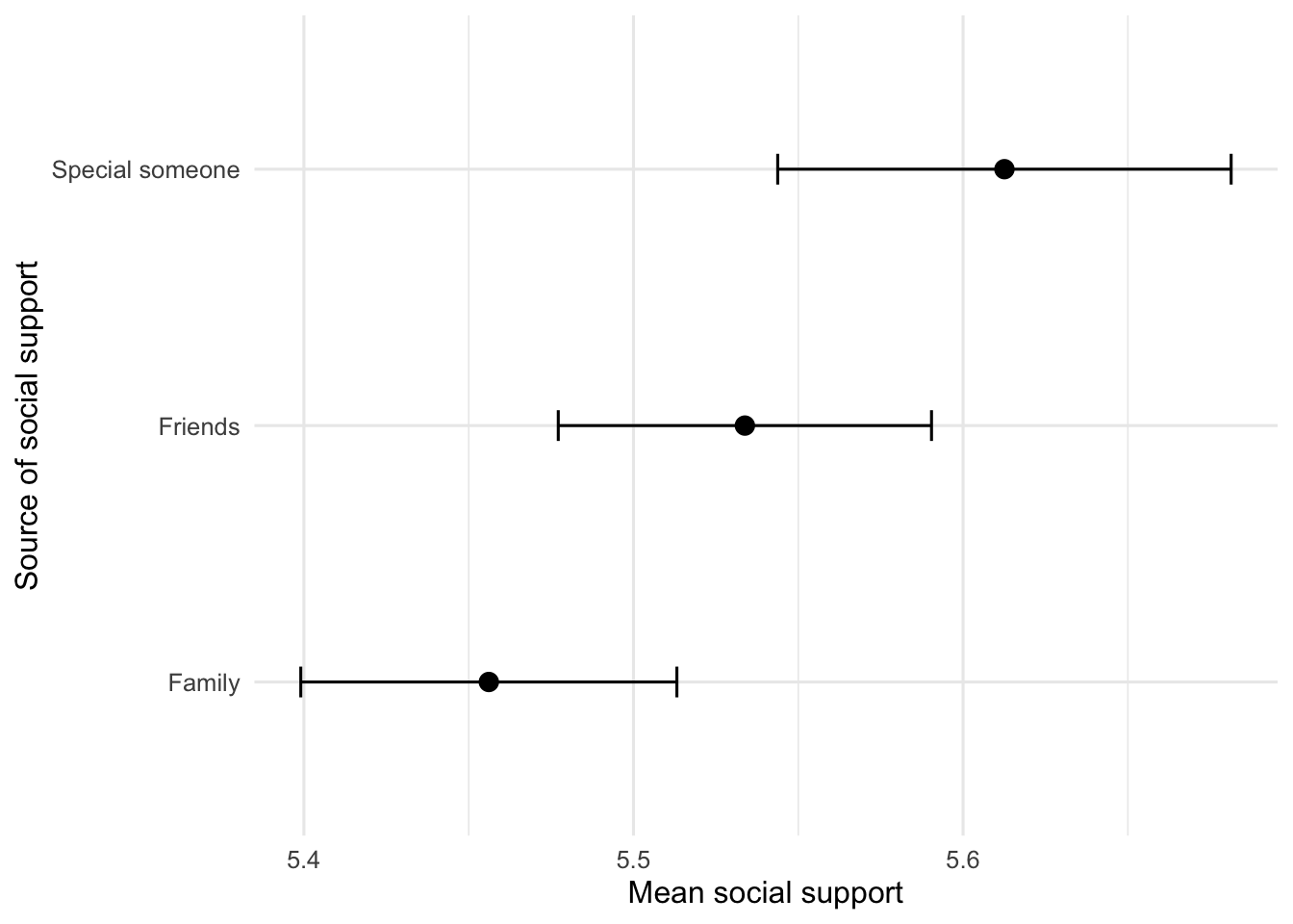
A repeated-measures ANOVA revealed significant differences in reported support, F(2, 4140) = 11.47, p < .001, partial η² = .006. Support was highest from a special someone (M = 5.61, SE = 0.04), followed by friends (M = 5.53, SE = 0.03), and family (M = 5.46, SE = 0.03). Friends were significantly higher than family, p = .008, d = 0.07. A special someone was higher than family, p < .001, d = 0.15. Support from a special someone and friends did not significantly differ, p = .059, d = 0.07.
NoteCareful interpretation
These are measured responses from the same participants. We can say reported support differs across sources, but not that the source caused the difference.
Chapter Takeaway
A repeated-measures ANOVA compares three or more related means and accounts for the fact that each participant contributes multiple scores. Wide data store repeated scores in separate variables; long data identify the condition and score in separate columns.
R Skills Practiced
row_number()creates a participant number for each observation.pivot_longer()reshapes repeated scores from wide to long format.factor(Participant)identifies participant labels in the model.repeated_eta_squared()calculates partial eta squared.repeated_pairwise_tests()is supplied by the setup file and compares each pair of repeated scores.